Introduction

The reorder point is the level of inventory at which an order is placed. If the demand rate is a known constant, then the reorder point is:

\[ \text{ Reorder Point} = \text{ demand rate}\times \text{ lead time} \]

where \(\text{ lead time}\) is the amount of time between the placement of an order and its receipt (assumed constant as well here).

For example, if the demand rate is 10 units/day and the lead time is 5 days, then the Reorder Point is going to be 50 units.

When the demand is stochastic and/or the lead time is stochastic, the lead-time demand is stochastic and, thus, a stockout is possible.

For example:

• Stochastic demand and constant lead time: suppose the daily demand fluctuates among 9, 10 and 11 units and the lead time is 5 days. Then the lead-time demand is stochastic falling somewhere in the interval between 45 and 55.

• Constant demand and stochastic lead time: suppose the daily demand is always 10 units per day, and the lead time fluctuates among 4, 5 and 6 days. Then the lead-time demand is stochastic, fluctuating among 40, 50 and 60 units.

• Stochastic demand and stochastic lead time: suppose the daily demand fluctuates amoing 9, 10 and 11 units, and the lead time fluctuates among 4, 5 and 6 days. Then the lead-time demand is stochastic, falling somewhere between 36 and 66 units.

So, if we use a reorder point of 50 units, mentioned in the example above, as the reorder point, a stockout will occur whenever the lead-time demand exceeds 50 units.

Stochastic Demand and Stochastic Lead Time

The reoder point when the demand and the lead time are stochastic is:

\(ROP = \text{Expected demand during lead time} + \text{Safety Stock}\)

The safety stock serves to reduce the probability of experiencing a stockout during lead time.

• Safety stock (SS): stock that is held in excess of expected demand due to variable demand rate and/or variable lead time.

To be able to calculate the safety stock, one approach is to define a service level which is the probability that the demand will not excess supply during lead time. Formally:

\[\text{Service Level (SL)} = P(D_L < ROP)\]

where, \(D_L\) is the lead-time demand.

With these definitions, we can start to create a probabilistic model to calculate the reorder point:

• Assumptions:

  • The demands are i.i.d random variables
  • The demands are independent of the lead time

• For explanation, we will assume that we have daily demands

• The amount of safety stock depends on:

  • The desired service level
  • The daily demand denoted \(D_i\) with unit in items/per day and let’s suppose that the average and standard deviation of the daily demand \(D_i\) are \((\mu_D, \sigma_D)\)
  • The lead time denoted \(L\) with unit in number of days and let’s suppose the average and standard deviation of the lead time are \((\mu_L, \sigma_L)\)

• The lead-time demand (demand during lead time) is now another random variable:

\[D_L = \sum_{i = 1}^{L} D_i = D_1 + D_2 + \dots + D_L\]

To construct the ROP, let’s first calculate the expected demand during the lead time \(E(D_L)\). The tricky part of getting the expectation (as well the standard deviation) of \(D_L\) is that the lovely \(L\) is a random variable (in the summation) otherwirse it would be trivial.

I will derive the \(E[D_L]\) and \(\sigma(D_L)\) instead of throwing to you the formulas. To do so, we need the Total Expectation Theorem:

\[E(X) = \sum_{y} E(X \mid Y = y) \cdot P(Y = y)\]

Proof:

\[\begin{align} E(X) &= \sum_{y} E(X \mid Y = y) \cdot P(Y = y) \\ &= \sum_{y}\sum_{x}x \cdot P(X=x \mid Y=y) \cdot P(Y=y) \\ &= \sum_{y}\sum_{x}x \cdot \frac{P(X=x, Y=y)}{P(Y=y)} \cdot P(Y=y) \\ &= \sum_{y}\sum_{x}x \cdot P(X=x, Y=y) \\ &= \sum_{x}x \sum_{y}P(X=x, Y=y) \\ &= \sum_{x}x \cdot P(X=x) \\ &= E(X) \end{align}\]

Derivation of \(E(\sum_{i = 1}^{L} D_i)\) :

\[\begin{align} E(\sum_{i=1}^{L}D_i) &= \sum_{l=1}^{L}E(\sum_{i=1}^{L}D_i \mid L = l) \cdot P(L = l) \\ &= \sum_{l=1}^{L}E(\sum_{i=1}^{l}D_i) \cdot P(L = l) \\ &= \sum_{l=1}^{L}l \cdot \mu_D \cdot P(L = l) \\ &= \mu_D \cdot \sum_{l=1}^{L}l \cdot P(L = l) \\ &= \mu_D \cdot \mu_L \end{align}\]

Derivation of \(VAR(\sum_{i = 1}^{L} D_i)\). I will use the definition of the variance \(VAR(X) = E(X^2) . (E(X))^2\) :

\[\begin{align} VAR(\sum_{i=1}^{L}D_i) &= E((\sum_{i=1}^{L}D_i)^2) - (E(\sum_{i=1}^{L}D_i))^2 \end{align}\]

For the first term, we have:

\[\begin{align} E((\sum_{i=1}^{L}D_i)^2) &= \sum_{l=1}^{L}E((\sum_{i=1}^{L}D_i)^2 \mid L = l) \cdot P(L = l) \\ &= \sum_{l=1}^{L}E((\sum_{i=1}^{l}D_i)^2) \cdot P(L = l) \\ &= \sum_{l=1}^{L}\big[ VAR(\sum_{i=1}^{l}D_i) + (E(\sum_{i=1}^{l}D_i))^2 \big] \cdot P(L = l) && \text{by definition of VAR(X)} \\ &= \sum_{l=1}^{L}\big[ l \cdot \sigma_D^2 + (l \cdot \mu_D)^2 \big] \cdot P(L = l) \\ &= \sum_{l=1}^{L}l \cdot \sigma_D^2 \cdot P(L = l) + \sum_{l=1}^{L}(l \cdot \mu_D)^2 \cdot P(L = l) \\ &= \sigma_D^2 \cdot \mu_L + \mu_D^2 \cdot E(L^2) \end{align}\]

Now, replacing this term in the original equation:

\[\begin{align} VAR((\sum_{i=1}^{L}D_i)^2) &= \sigma_D^2 \cdot \mu_L + \mu_D^2 \cdot E(L^2) - (E(\sum_{i=1}^{L}D_i))^2 \\ &= \sigma_D^2 \cdot \mu_L + \mu_D^2 \cdot E(L^2) - \mu_D^2 \cdot \mu_L \\ &= \sigma_D^2 \cdot \mu_L + \mu_D^2 \cdot (E(L^2) - \mu_L) \\ &= \sigma_D^2 \cdot \mu_L + \mu_D^2 \cdot \sigma_L^2 \end{align}\]

Now, let’s assume that \(D_L\) follows a normal distribution:

\(D_L \sim N(E(D_L), \sqrt{VAR(D_L)})\)

Above we defined the service level as:

\[\text{Service Level (SL)} = P(D_L < ROP)\] If we want to have a service level of 95%, meaning that we do not want to stockout 95% of the time (for example if we have 20 replenishments in a year, we expect to have only 1 stockout out of 20), then the formula becomes:

\[\text{0.95} = P(D_L < ROP)\]

\(D_L\) is a normal random variable, so we can use R to calculate the ROP that makes the service level equal to 95% (quantile function for the normal distribution):

\[ROP = qnorm(0.95, \ \text{mean =} E(D_L), \ \text{sd =} \sqrt{VAR(D_L)}, \ \text{lower.tail = TRUE})\]

And we know:

\[\begin{align} ROP &= \text{Expected demand during lead time} + \text{Safety Stock} \\ &= E(D_L) + \text{Safety Stock} \end{align}\]

Therefore the safety stock is:

\[\text{Safety Stock} = ROP - E(D_L)\]

Nonnormal Distributions

The first thing to notice is that \(E(D_L) \text{ and} \ VAR(D_L)\) do not assume any distributions. Hence, if the demand during lead time does not follow a normal distribution, we can do some of the following:

• We may use other distribution with those values (\(E(D_L) \text{ and} \ VAR(D_L)\)). Maybe I will cover this in a future post
• You are lucky enough that have historical demand during lead time, you can just find the quantile at certain service level
  • Or try to find the best distribution that fit your data, and then use the quantile for that distribution like we did for the normal case.

# Let's generate 10,000 lead-time demand from a Poisson Distribution with 
# parameter lambda equal to 50

library(ggplot2)

x = rpois(10000, lambda = 50)
x_df = data.frame(x)

ggplot(x_df, aes(x)) + geom_histogram(bins = 30) + theme_minimal() +
  labs(title = "Demand During Lead Time", subtitle = "Simulated Data",
       x = "demand")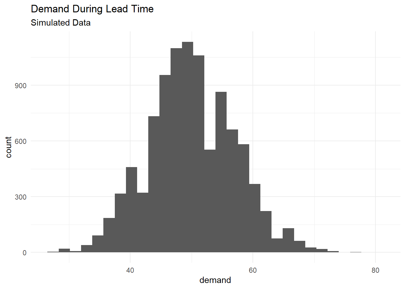

cat("ROP at 95% service level: ", quantile(x, probs = c(0.95)))

## ROP at 95% service level:  62

• Another possibility is to bootstrap. To do so, we need to have historical demands and historical lead times. The idea is simple:
  • Step 1: sample with replacement a lead time from the historical lead times bucket
  • Step 2: sample with replacement from the historical demands bucket an equal quantity of demands based on the lead time from Step 1. For example, in Step 1 we sample a lead time equal to 10 days, then we sample 10 demands from the historical demands (of course, the demands have to be in the same temporal units, in this case lead times are in days and demands are in units/days). Then you just sum those demands and that it is your first lead-time demand in the simulation.
  • Step 3: repeat 1 and 2 many times
  • Step 4: calculate quantile

Bootstrap

library(ggplot2)

set.seed(1)

# monthly demands for a spare part
month <- 1:24
demand <- c(0,0,8,2,0,0,0,35,0,0,0,5,10,0,0,3,0,16,0,0,0,8,0,0)

# simulate 6 lead times
LT <- sample(x = c(2, 3, 4), prob = c(0.15, 0.7, 0.15), size = 6, replace = TRUE)

# demand data frame
spare <- data.frame(month = month, demand = demand)

# we will run 25,000 simulations
ITER = 25000
LTD <- vector()

for(i in 1:ITER){
  lead_time <- sample(LT, size = 1)
  demand_sample <- sample(x = demand, replace = TRUE, size = lead_time)
  LTD[i] <- sum(demand_sample)
}

qplot(LTD, geom="histogram", bins=30) + theme_minimal() +
  labs(title = "25,000 Bootstrap Distribution",
       subtitle = "Spare Part",
       caption = "Source: Own Fake Data", 
       x = "Lead-Time Demand", y = "")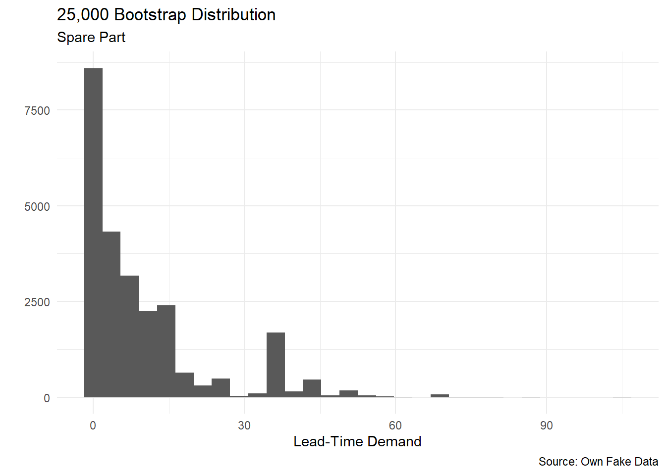 

cat("ROP at 80% service level: ", quantile(LTD, probs = c(0.80)), '\n')
cat("ROP at 90% service level: ", quantile(LTD, probs = c(0.90)), '\n')
cat("ROP at 95% service level: ", quantile(LTD, probs = c(0.95)), '\n')
cat("ROP at 99% service level: ", quantile(LTD, probs = c(0.99)))

## ROP at 80% service level:  16 
## ROP at 90% service level:  35 
## ROP at 95% service level:  37 
## ROP at 99% service level:  51

This example tries to show an example for a spare part. Out of the 24 months of historical demand, we have 16 months with 0 demand. Now, when you need to decide your reorder point, you have to consider if the product is critical for the operation of your business. If the spare part is very expensive but not critical may be a good idea to have a lower service level. Less money ties on inventory reduces working capital. On the other hand, if the spare part is super critical and all your operations can shut down because of not having it available, you may probably go with a high service level of 95% or 99%.