Introduction

Loess is a class of regression models that allows us to estimate the regression function $f\left(X\right)$ by fitting a simple (and different) model to each point in the domain $X$. This is done by paying attention to the points closest to a particular target point $x_0\in X$.

In the classic simple linear regression we have the following model:

$$y_i=f\left(x_i\right)+{ϵ}_i$$

where $f\left(x_i\right)$ is:

$$f\left(x_i\right)={\beta }_0+{\beta }_1\cdot x_i$$ and in the case of loess with approximate $f\left(x_i\right)$ by a polynomial weigthed by a function $w_i$ that assigns higher weights to points $x_i$ that are closer to $x_0$:

$$f\left(x_i\right)=w_i\left(x_0\right)\cdot [{\beta }_0+{\beta }_1\cdot x_i+{\beta }_2\cdot x_i^2+\dots ]$$

Procedure:

0. Let $x_i$ denote a set of $n$ values for a particular variable and let $y_i$ represent the corresponding response variable.

1. Find the $k$ closest points to the target point $x_0$. Let’s denote this set $D_0$

   • For implementation, keep track of these points and their distances $d_{i0}$

2. Find the furthest distance among those $k$ points. Let’s denote this quantity as $\delta \left(x_0\right)$

3. Calculate the weight function $w_i$ for each $x_i\in D_0$ using the tricube weight function:

$$w_i\left(x_0\right)=W\left(\frac{d_{i0}}{\delta \left(x_0\right)}\right)$$

where $W(\cdot )$:

$$W\left(u\right)=\{\begin{array}{cc}(1-u^3{)}^3,& 0\le u<1\\ 0,& \text{otherwise}\end{array}$$

4. Calculate the prediction $\hat{f}\left(x_0\right)$ by solving weigthed least squares. The normal equation can be expressed as followed:

$$\begin{array}{cc}WX\hat{\beta }& =Wy\\ X^{\prime }WX\hat{\beta }& =X^{\prime }Wy\\ \hat{\beta }& =(X^{\prime }WX{)}^{-1}{X}^{\prime }Wy\end{array}$$

• You need to use only the $k$ closest points for each target point $x_0$

  • In the case of a polynomial of degree 1:
    • W is a 2x2 diagonal matrix
    • X is a kx2 matrix (column 1 it is a column of 1’s for the intercept)
    • y is a kx1 vector
  • In the case of a polynomial of degree 2:
    • W is a 3x3 diagonal matrix
    • X is a kx3 matrix
    • y is a kx1 vector

• With the estimates of $\hat{\beta }$ you can calculate $\hat{f}\left(x_0\right)$

Implementation

In the implementation, I included an option to not use all the $x_i$ points as $x_0$ because when there are many samples, the fit takes long time.

Also, to solve the normal equation above, I did a QR decomposition for stability 1.

import numpy as np
import pandas as pd
import matplotlib.pyplot as plt
import seaborn as sns
from scipy.linalg import qr, pinv
from scipy.linalg import solve_triangular


def loess(X, y, alpha, deg, all_x = True, num_points = 100):
    '''
    Parameters
    ----------
    X : numpy array 1D
        Explanatory variable.
    y : numpy array 1D
        Response varible.
    alpha : double
        Proportion of the samples to include in local regression.
    deg : int
        Degree of the polynomial to fit. Option 1 or 2 only.
    all_x : boolean, optional
        Include all x points as target. The default is True.
    num_points : int, optional
        Number of points to include if all_x is false. The default is 100.

    Returns
    -------
    y_hat : numpy array 1D
        Y estimations at each focal point.
    x_space : numpy array 1D
        X range used to calculate each estimation of y.

    '''
    
    assert (deg == 1) or (deg == 2), "Deg has to be 1 or 2"
    assert (alpha > 0) and (alpha <=1), "Alpha has to be between 0 and 1"
    assert len(X) == len(y), "Length of X and y are different"
    
    if all_x:
        X_domain = X
    else:
        minX = min(X)
        maxX = max(X)
        X_domain = np.linspace(start=minX, stop=maxX, num=num_points)
        
    n = len(X)
    span = int(np.ceil(alpha * n))
    #y_hat = np.zeros(n)
    #x_space = np.zeros_like(X)
    
    y_hat = np.zeros(len(X_domain))
    x_space = np.zeros_like(X_domain)
    
    for i, val in enumerate(X_domain):
    #for i, val in enumerate(X):
        distance = abs(X - val)
        sorted_dist = np.sort(distance)
        ind = np.argsort(distance)
        
        Nx = X[ind[:span]]
        Ny = y[ind[:span]]
        
        delx0 = sorted_dist[span-1]
        
        u = distance[ind[:span]] / delx0
        w = (1 - u**3)**3
        
        W = np.diag(w)
        A = np.vander(Nx, N=1+deg)
        
        V = np.matmul(np.matmul(A.T, W), A)
        Y = np.matmul(np.matmul(A.T, W), Ny)
        Q, R = qr(V)
        p = solve_triangular(R, np.matmul(Q.T, Y))
        #p = np.matmul(pinv(R), np.matmul(Q.T, Y))
        #p = np.matmul(pinv(V), Y)
        y_hat[i] = np.polyval(p, val)
        x_space[i] = val
        
    return y_hat, x_space

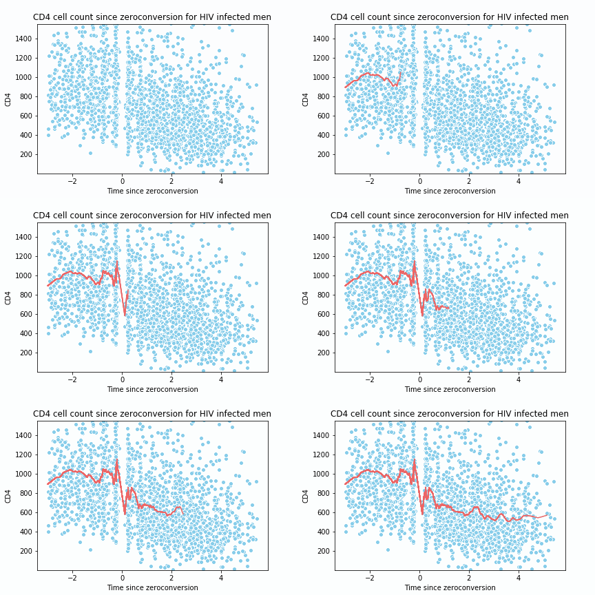
To test the implementation and create the animation, I replicate the following lecture notes 2. The dataset is located here 3.

import matplotlib.animation as animation
from matplotlib.animation import FuncAnimation, PillowWriter

c4 = pd.read_csv("cd4.data.txt", delim_whitespace=True, header=None)
y_hat2, x_space2 = loess(c4[0], c4[1], 0.05, 1, all_x = True, num_points = 200)

d = {'x': x_space2, 'y': y_hat2}
c4_pred = pd.DataFrame(data = d)
c4_pred = c4_pred.sort_values(by = ['x'])
c4_pred = c4_pred.reset_index(drop=True)

def animate(i):
    x_data = c4_pred.x.values[:i]
    y_data = c4_pred.y.values[:i]
    #sns.scatterplot(c4[0], c4[1], color ='skyblue')
    sns.lineplot(x= x_data, y=y_data, color = '#EE6666')

fig = plt.figure()
sns.scatterplot(c4[0], c4[1], color ='skyblue')
plt.ylim(1, 1550)
plt.xlabel("Time since zeroconversion")
plt.ylabel("CD4")
plt.title("CD4 cell count since zeroconversion for HIV infected men")

writer = animation.PillowWriter()

ani = FuncAnimation(fig, animate, frames = np.arange(0, 2376, 40))
ani.save('ani_cd4.gif', writer=writer)